How to Conduct Multiple Linear Regression
Multiple Linear Regression Analysis involves more than just drawing a line through data points. It has three main steps:
(1) examining the data’s correlation and direction.
(2) fitting the line to the model, and
(3) assessing the model’s validity and usefulness.
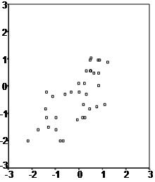
Start by analyzing scatter plots for each independent variable to check the data’s direction and correlation. For instance, the first scatter plot we show demonstrates a positive relationship between two variables.
The data fits the requirements to run a multiple linear regression analysis.
Need help conducting your Multiple Linear Regression? Leverage our 30+ years of experience and low-cost same-day service to make progress on your results today!
Schedule now using the calendar below.
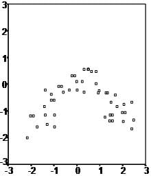
The second scatter plot seems to have an arch-shape this indicates that a regression line might not be the best way to explain the data, even if a correlation analysis establishes a positive link between the two variables. However, most often data contains quite a large amount of variability (just as in the third scatter plot example) in these cases it is up for decision how to best proceed with the data.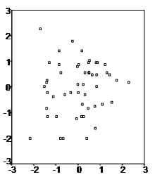
The second step of multiple linear regression is to formulate the model, i.e. that variable X1, X2, and X3 have a causal influence on variable Y and that their relationship is linear.
The third step of regression analysis is to fit the regression line.
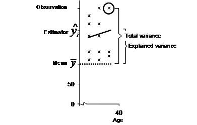
Least squares estimation minimizes the unexplained residuals. The following graph illustrates the basic idea behind this concept.
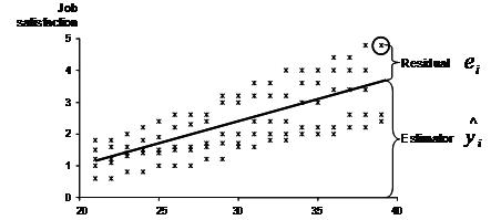
In our example we want to model the relationship between age, job experience, and tenure on one hand and job satisfaction on the other hand. The research team has gathered several observations of self-reported job satisfaction and experience, as well as age and tenure of the participant.
Fitting a line through the scatter plot estimates job satisfaction based on the input factors. However in most cases the real observation might not fall exactly on the regression line.
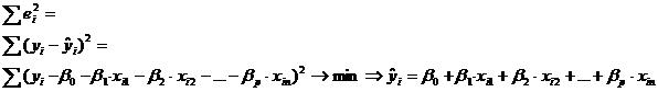
Because we try to explain the scatter plot with a linear equation of![]()
for i = 1…n. The deviation between the regression line and the single data point is variation that our model can not explain. The unexplained variation refers to the residual, .
The method of least squares is used to minimize the residual.
The multiple linear regression’s variance ![]() is estimated by
is estimated by

where p is the number of independent variables and n the sample size.
The result of this equation could for instance be yi = 1 + 0.1 * xi1+ 0.3 * xi2 – 0.1 * xi3+ 1.52 * xi4. This means that for additional unit x1 (ceteris paribus) we would expect an increase of 0.1 in y, and for every additional unit x4 (c.p.) we expect 1.52 units of y.
Now that we got our multiple linear regression equation we evaluate the validity and usefulness of the equation.
The key measure to the validity of the estimated linear line is R². R² = total variance / explained variance. The following graph illustrates the key concepts to calculate R². In our example the R² is approximately 0.6, this means that 60% of the total variance is explained with the relationship between age and satisfaction.
As you can easily see the number of observations and of course the number of independent variables increases the R². Overfitting occurs in multiple linear regression when the model becomes inefficient. To identify whether the multiple linear regression model is fitted efficiently a corrected R² is calculated (it is sometimes called adjusted R²), which is defined
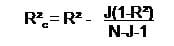
where J is the number of independent variables and N the sample size. As you can see the larger the sample size the smaller the effect of an additional independent variable in the model.
In our example R²c = 0.6 – 4(1-0.6)/95-4-1 = 0.6 – 1.6/90 = 0.582. Thus we find the multiple linear regression model quite well fitted with 4 independent variables and a sample size of 95.
The last step for the multiple linear regression analysis is the test of significance. Multiple linear regression uses two tests to check if the model and coefficients apply to the general population. Firstly, the F-test tests the overall model. The null hypothesis is that the independent variables have no influence on the dependent variable. In other words the F-tests of the multiple linear regression tests whether the R²=0. Secondly, multiple t-tests analyze the significance of each individual coefficient and the intercept. The t-test has the null hypothesis that the coefficient/intercept is zero.