Conduct and Interpret a Cluster Analysis
What is Cluster Analysis?
Cluster analysis is a versatile and exploratory data analysis technique used to identify natural groupings or clusters within a dataset. It is also known as segmentation analysis or taxonomy analysis and is particularly useful when the groupings within data are not previously known. This technique is exploratory in nature, focusing solely on discovering and describing structures and patterns in the data without distinguishing between dependent and independent variables.
Applications of Cluster Analysis
Cluster analysis is applied across various fields to uncover distinct groups based on similarities within the data. Here are a few examples:
Medicine: Used to identify diagnostic clusters by analyzing patient symptoms to group similar cases. For instance, in psychology, cluster analysis might classify patients with similar behavioral patterns, aiding in targeted treatment plans.
Marketing: Helps in market segmentation by analyzing consumer data such as needs, attitudes, demographics, and behaviors. This can inform targeted marketing strategies by identifying customer segments with similar characteristics.
Education: It identifies groups of students requiring specific educational interventions by analyzing psychological, aptitude, and achievement data. As a result, this analysis can help in developing tailored educational programs and support.
Need help conducting your Cluster Analysis? Leverage our 30+ years of experience and low-cost same-day service to complete your results today!
Schedule now using the calendar below.
Biology: Assists in creating taxonomies by clustering species based on phenotypic characteristics. This can lead to a better understanding of biodiversity and ecosystem relationships.
Data Preparation: Ensure data is properly cleaned and preprocessed. This includes handling missing values, normalizing data, and selecting the appropriate variables for analysis.
Choosing the Right Method: Select a clustering method that best fits the data type and the nature of the analysis. SPSS, for example, offers various methods that can handle different data types, including binary, nominal, ordinal, and scale (interval or ratio).
Determining the Number of Clusters: Techniques such as the elbow method, silhouette analysis, or hierarchical clustering can help in determining the optimal number of clusters.
Running the Analysis: Use software like SPSS to perform the cluster analysis. Configure the specific parameters such as distance metrics and linkage criteria based on the chosen method.
Interpreting Results: Analyze the output to understand the characteristics of each cluster. Assess the clusters for validity and reliability based on the coherence and differences between the groups.
Complementary Techniques
Q-analysis and Multi-dimensional Scaling (MDS): You can also use these techniques to explore data structures and identify groupings based on different criteria or dimensions.
Latent Class Analysis (LCA): It offers a probabilistic approach to grouping data based on latent class membership, making it useful in more complex structures where variables interrelate.
Conclusion
Cluster analysis is a powerful tool for uncovering hidden patterns and structures in data across various domains. By effectively grouping similar observations, it enables researchers and analysts to derive meaningful insights and make informed decisions. Whether in marketing, medicine, education, or biology, cluster analysis provides a foundation for deeper understanding and targeted action.
The Cluster Analysis in SPSS
Our research question for this example cluster analysis is as follows:
What homogenous clusters of students emerge based on standardized test scores in mathematics, reading, and writing?
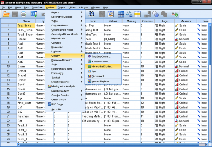
In SPSS Cluster Analyses can be found in Analyze/Classify…. SPSS offers three methods for the cluster analysis: K-Means Cluster, Hierarchical Cluster, and Two-Step Cluster.
K-means cluster is a method to quickly cluster large data sets. The researcher define the number of clusters in advance. This is useful to test different models with a different assumed number of clusters.
Hierarchical cluster is the most common method. It generates a series of models with cluster solutions from 1 (all cases in one cluster) to n (each case is an individual cluster). Hierarchical cluster also works with variables as opposed to cases; it can cluster variables together in a manner somewhat similar to factor analysis. In addition, hierarchical cluster analysis can handle nominal, ordinal, and scale data; however it is not recommended to mix different levels of measurement.
Two-step cluster analysis identifies groupings by running pre-clustering first and then by running hierarchical methods. Because it uses a quick cluster algorithm upfront, it can handle large data sets that would take a long time to compute with hierarchical cluster methods. In this respect, it is a combination of the previous two approaches. Two-step clustering can handle scale and ordinal data in the same model, and it automatically selects the number of clusters.
Hierarchical Cluster Analysis Steps
The hierarchical cluster analysis follows three basic steps: 1) calculate the distances, 2) link the clusters, and 3) choose a solution by selecting the right number of clusters.
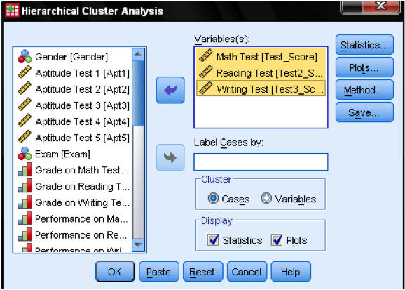
First, we have to select the variables upon which we base our clusters. In the dialog window we add the math, reading, and writing tests to the list of variables. Since we want to cluster cases we leave the rest of the tick marks on the default.
Step 2
In the dialog box Statistics… we can specify whether we want to output the proximity matrix (these are the distances calculated in the first step of the analysis) and the predicted cluster membership of the cases in our observations. Again, we leave all settings on default.
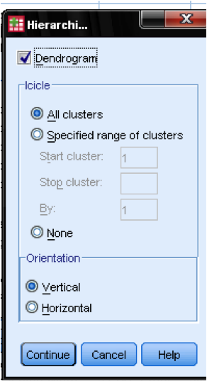
In the dialog box Plots… we should add the Dendrogram. The Dendrogram graphically shows how the clusters merge and helps identify the appropriate number of clusters.
Dialog box Method
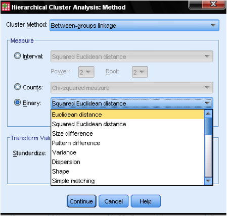
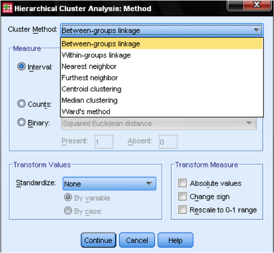
The dialog box Method… allows us to specify the distance measure and the clustering method. First, we need to define the correct distance measure. SPSS offers three large blocks of distance measures for interval (scale), counts (ordinal), and binary (nominal) data.
For interval data, the most common is Square Euclidian Distance. It is based on the Euclidian Distance between two observations, which is the square root of the sum of squared distances. Since the Euclidean distance squares the values, it increases the importance of large distances while reducing the impact of small distances.
If we have ordinal data (counts) we can select between Chi-Square or a standardized Chi-Square called Phi-Square. For binary data, the Squared Euclidean Distance is commonly used.
In our example, we choose Interval and Square Euclidean Distance.
Next, we have to choose the Cluster Method. Typically, choices are between-groups linkage (distance between clusters is the average distance of all data points within these clusters), nearest neighbor (single linkage: distance between clusters is the smallest distance between two data points), furthest neighbor (complete linkage: distance is the largest distance between two data points), and Ward’s method (distance is the distance of all clusters to the grand average of the sample). Single linkage works best with long chains of clusters, while complete linkage works best with dense blobs of clusters. Between-groups linkage works with both cluster types. It is recommended is to use single linkage first. Although single linkage tends to create chains of clusters, it helps in identifying outliers. After excluding these outliers, we can move onto Ward’s method. Ward’s method uses the F value (like in ANOVA) to maximize the significance of differences between clusters.
A last consideration is standardization. If the variables have different scales and means we might want to standardize either to Z scores or by centering the scale. We can also transform the values to absolute values if we have a data set where this might be appropriate.
