Assumptions of Multiple Linear Regression
Multiple Regression With Multicollinearity Is Garbage In, Garbage Out. Your Committee Checks VIF Before Anything Else.
Everything that applies to simple linear regression applies here: linearity, normality of residuals, homoscedasticity, independence. But multiple regression adds one assumption that can quietly destroy your entire analysis: multicollinearity. When your predictors are too highly correlated with each other, your coefficients become unstable, your standard errors inflate, and your results can flip sign without warning. Your committee knows this. They’ll look at your VIF values before they look at your p-values.
The tipping point in multiple regression isn’t the R². It’s the VIF table. A VIF above 5 raises eyebrows. A VIF above 10 raises objections. And no amount of significant predictors can save a model built on collinear variables.
Check your VIF. Report it. Address any issues transparently. That one table can be the tipping point between a Chapter 4 that sails through and one that sinks.

Get Expert Help with Your Results. Schedule Your Free Consultation.
20 minutes with Dr. Lani. No obligation. No pressure.
Multiple linear regression analysis is based on several fundamental assumptions that ensure the validity and reliability of its results. Understanding and checking these assumptions is crucial for accurate model interpretation and prediction.
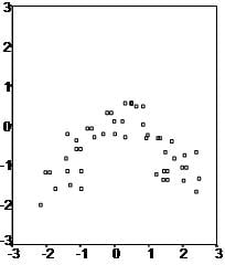
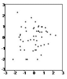
Linear Relationship: The core premise of multiple linear regression is the existence of a linear relationship between the dependent (outcome) variable and the independent variables. One can view this linearity visually using scatterplots, which should reveal a linear relationship rather than a curvilinear one.
Multivariate Normality: The analysis assumes that the unclear variations (the differences between viewed and predicted values) are normally provided. This assumption can be vague by examining histograms or Q-Q plots of the residuals, or through statistical tests such as the Kolmogorov-Smirnov test.
No Multicollinearity: It is essential to avoid high correlation between the independent variables, a condition known as multicollinearity. This can be checked using:
Correlation matrices, where correlation coefficients should ideally be below 0.80.
Variance Inflation Factor (VIF), with VIF values above 10 indicating problematic multicollinearity. Solutions may include centering the data (subtracting the mean score from each observation) or removing the variables causing multicollinearity.
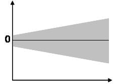
Homoscedasticity: The variance of error terms (residuals) should be consistent across all levels of the independent variables. A scatterplot of residuals versus predicted values should not display any discernible pattern, such as a cone-shaped distribution, which would indicate heteroscedasticity. Addressing heteroscedasticity might involve data transformation or adding a quadratic term to the model.
Sample Size and Variable Types: The model requires at least two independent variables, which can be of nominal, ordinal, or interval/ratio scale. A general guideline for sample size is a minimum of 20 cases per independent variable.
Multiple Linear Regression Assumptions
First, multiple linear regression requires the relationship between the independent and dependent variables to be linear. One can test the linearity assumption best with scatterplots. The following two examples depict a curvilinear relationship (top image) and a linear relationship (bottom image).
Second, the multiple linear regression analysis requires that the errors between observed and predicted values (i.e., the residuals of the regression) follow a normal distribution. One can check this assumption by looking at a histogram or a Q-Q plot. One can check normality with a goodness of fit test (e.g., Kolmogorov-Smirnov) on the residuals.
Third, multiple linear regression assumes that there is no multicollinearity in the data. Multicollinearity occurs when the independent variables become too highly correlated with each other.
You can check for multicollinearity in multiple ways:
1) Correlation matrix – When computing a matrix of Pearson’s bivariate correlations among all independent variables, the magnitude of the correlation coefficients should be less than .80.
2) Variance Inflation Factor (VIF) – The VIFs of the linear regression indicate the degree that the variances in the regression estimates are increased due to multicollinearity. VIF values higher than 10 indicate that multicollinearity is a problem.
If multicollinearity is found in the data, one possible solution is to center the data. To center the data, subtract the mean score from each observation for each independent variable. However, the simplest solution is to identify the variables causing multicollinearity issues (i.e., through correlations or VIF values) and removing those variables from the regression.
The last assumption of multiple linear regression is homoscedasticity. A scatterplot of residuals versus predicted values is good way to check for homoscedasticity. There should be no clear pattern in the distribution; if there is a cone-shaped pattern (as shown below), the data is heteroscedastic.
If the data are heteroscedastic, a non-linear data transformation or addition of a quadratic term might fix the problem.