The Logistic Regression Analysis in SPSS

Our example is a research study on 107 pupils. We measured these pupils using five different aptitude tests, one for each important category (reading, writing, understanding, summarizing, etc.). The question now is – How do these aptitude tests predict if the pupils passes the year end exam?

First, we need to check that we populate all cells in our model. Although the logistic regression is robust against multivariate normality and therefore better suited for smaller samples than a probit model, we still need to check, because we don’t have any categorical variables in our design we will skip this step.

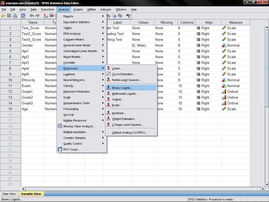
Logistic Regression is found in SPSS under Analyze/Regression/Binary Logistic…

This opens the dialogue box to specify the model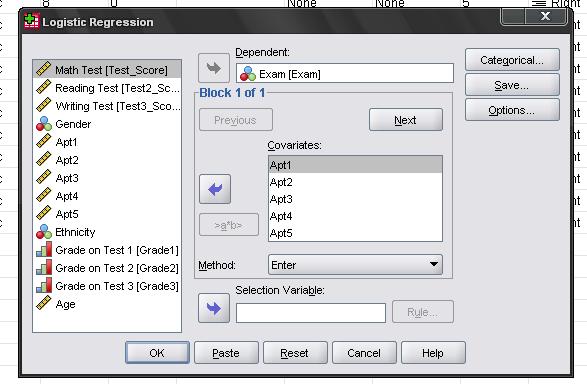

Here we need to enter the nominal variable Exam (pass = 1, fail = 0) into the dependent variable box and we enter all aptitude tests as the first block of covariates in the model.

The menu categorical… allows to specify contrasts for categorical variables (which we do not have in our logistic regression model), and options offers several additional statistics, which don’t need.

The first table just shows the sample size.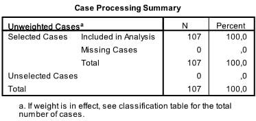

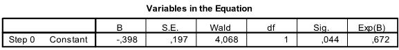
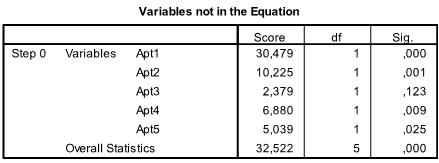
The next 3 tables are the results fort he intercept model. That is the Maximum Likelihood model, which includes only the intercept and excludes any dependent variables from the analysis. This is basically only interesting to calculate the Pseudo R² that describe the goodness of fit for the logistic model.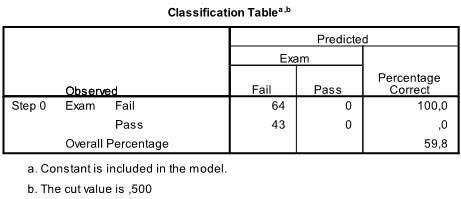

The relevant tables are in the ‘Block 1’ section of the SPSS output for our logistic regression analysis. The first table includes the Chi-Square goodness of fit test. It has the null hypothesis that intercept and all coefficients are zero. We can reject this null hypothesis.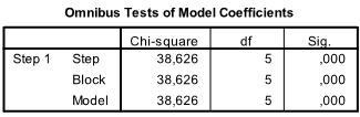

The next table includes the Pseudo R², with the -2 log likelihood serving as the minimization criteria used by SPSS. We see that Nagelkerke’s R² is 0.409 which indicates that the model is good but not great. Cox & Snell’s R² is the nth root (in our case the 107th of the -2log likelihood improvement. We can interpret this as the logistic model explaining a 30% probability of the event passing the exam.

The next table contains the classification results, with almost 80% correct classification the model is not too bad – generally a discriminant analysis is better in classifying data correctly.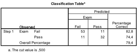

The last table is the most important one for our logistic regression analysis. It shows the regression function -1.898 + .148*x1 – .022*x2 – .047*x3 – .052*x4 + .011*x5. The table also includes the test of significance for each of the coefficients in the logistic regression model. For small samples, t-values are invalid, so the Wald statistic should be used instead. Wald is essentially t², following a Chi-Square distribution with df = 1. However, SPSS gives the significance levels of each coefficient. As we can see, only Apt1 is significant all other variables are not.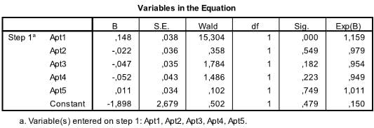

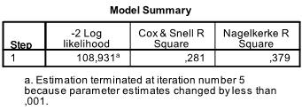
If we change the method from Enter to Forward:Wald the quality of the logistic regression improves. Now only the significant coefficients are included in the logistic regression equation. In our case this is Apt1 and the intercept.

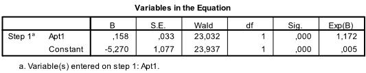
We see that , and we know that a 1 point higher score in the Apt1 test multiplies the odds of passing the exam by 1.17 (exp(.158)). We can also calculate the critical value which is Apt1 > -intercept/coefficient > -5.270/.158 > 33.35. That is if a pupil scored higher than 33.35 on the Aptitude Test 1 the logistic regression predicts that this pupil will pass the final exam.