How to Conduct Linear Regression
Linear Regression Analysis consists of more than just fitting a linear line through a cloud of data points. It consists of 3 stages – (1) analyzing the correlation and directionality of the data, (2) estimating the model, i.e., fitting the line, and (3) evaluating the validity and usefulness of the model.
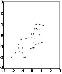
First, a scatter plot should be used to analyze the data and check for directionality and correlation of data. The first scatter plot indicates a positive relationship between the two variables. Researchers fit the data to run a regression analysis.
Need help conducting your Linear Regression Analysis? Leverage our 30+ years of experience and low-cost same-day service to complete your results today!
Schedule now using the calendar below.
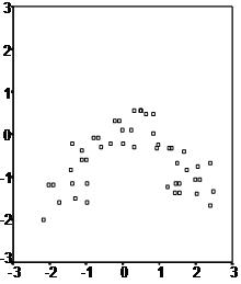
The second scatter plot seems to have an inverse U-shape this indicates that a regression line might not be the best way to explain the data, even if a correlation analysis establishes a positive link between the two variables.
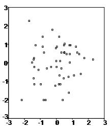
However, most often data contains quite a large amount of variability in these cases it is up for decision how to best proceed with the data.
The first step enables the researcher to formulate the model, i.e. that variable X has a causal influence on variable Y and that their relationship is linear.
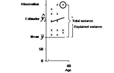
The second step of regression analysis is to fit the regression line. Researchers use least square estimation to minimize the unexplained residual. The following graph illustrates the basic idea behind this concept. In our example we want to model the relationship between age and job satisfaction. The research team has gathered several observations of self-reported job satisfaction and the age of the participant.
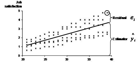
When we fit a line through the scatter plot, the regression line represents the estimated job satisfaction for a given age. However the real observation might not fall exactly on the regression line. We try to explain the scatter plot with a linear equation of y = b0 + b1x. The distance between the regression line and the data point represents the unexplained variation, which is also called the residual ei.
The method of least squares is used to minimize the residual.

The result of this equation would for instance be yi = 1 + 0.1 * xi. This means that for every year of age we would expect an increase of 0.1 in job satisfaction.
Now that we got our equation we evaluate the validity and usefulness of the equation. The key measure to the validity of the estimated linear line is R². R² = total variance / explained variance. The following graph illustrates the key concepts to calculate R². In our example, the R² is approximately 0.6; thus, the relationship between age and satisfaction explains 60% of the total variance.
As you can easily see the number of observations and of course the number of independent variables increases the R². However over-fitting occurs when the model is not efficient anymore. To identify whether the model fits efficiently, researchers calculate a corrected R², which they define as:
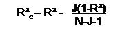
*J is the number of independent variables and N the sample size.
As you can see the larger the sample size the smaller the effect of an additional independent variable in the model. In our example R²c = 0.6 – 1(1-0.6)/95-1-1 = 0.5957. Thus the model is quite well fitted with only one independent variable in the analysis.
The last step for the linear regression analysis is the test of significance. Linear regression uses two tests to determine whether the model and the estimated coefficients apply to the general population from which researchers drew the sample. Firstly, the F-test tests the overall model. The null hypothesis is that the independent variables have no influence on the dependent variable. In other words the F-tests of the linear regression tests whether the R²=0. Secondly, multiple t-tests analyze the significance of each coefficient and the intercept. The t-test has the null hypothesis that the coefficient/intercept is zero.