Transforming Data for Normality
Normality is a common assumption in statistical analyses, with most parametric tests requiring it. Normality in regression refers to the error distribution, not individual variables. However, it’s easier to meet the assumption if each variable is normally distributed.. Let’s look at how we can make that happen.
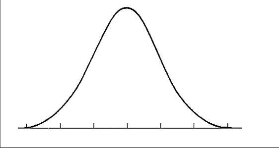
Often one of the first steps in assessing normality is to review a histogram of the variable in question. In this format, the X axis shows a variable’s values. And, the Y axis represents the number of participants with each value. A normal distribution has most of the participants in the middle, with fewer on the upper and lower ends – this forms a central “hump” with two tails. It should look something like this:
Need help conducting your analysis? Leverage our 30+ years of experience and low-cost same-day service to complete your results today!
Schedule now using the calendar below.
Sometimes, though, this is not what the data look like. A possible way to fix this is to apply a transformation. Transforming data is a method of changing the distribution by applying a mathematical function to each participant’s data value. If you have run a histogram to check your data and it looks like any of the pictures below, you can simply apply the given transformation to each participant’s value and attempt to push the data closer to a normal distribution.
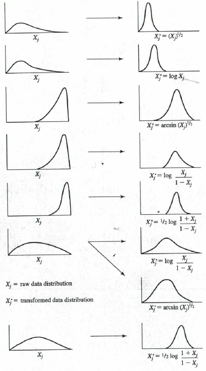
Figure from Stevens (2002) Applied Multivariate Statistics for the Social Sciences 5th ed.
For example, if your data looks like the top example, take everyone’s value for that variable and apply a square root (i.e., raise the variable to the ½ power). This is easy to do in a spreadsheet program like Excel and in most statistical software such as SPSS. You can then check the histogram again to see how the new variable compares to a normal distribution.
However, keep in mind that there is a bit of a tradeoff here. Your data may now be normal, but interpreting that data may be much more difficult. For example, if you run a t-test to check for differences between two groups, and the data you are comparing has been transformed, you cannot simply say that there is a difference in the two groups’ means. Now, you have the added step of interpreting the fact that the difference is based on the square root. For this reason, we usually try to avoid transformations unless necessary for the analysis to be valid.
For analyses like the F or t family of tests (i.e., independent and dependent sample t-tests, ANOVAs, MANOVAs, and regressions), violations of normality are not usually a death sentence for validity. As long as the sample size exceeds 30 (even better if it is greater than 50), there is not usually too much of an impact to validity from non-normal data; something that Stevens stressed in his 2016 publication of Applied Multivariate Statistics for the Social Sciences.