Conduct and Interpret an Ordinal Regression
What is Ordinal Regression?
Ordinal regression is a member of the family of regression analyses. As a predictive analysis, ordinal regression describes data and explains the relationship between one dependent variable and two or more independent variables. In ordinal regression analysis, the dependent variable is ordinal (statistically it is polytomous ordinal) and the independent variables are ordinal or continuous-level (ratio or interval).
Sometimes the dependent variable is also called response, endogenous variable, prognostic variable or regressand. The independent variables are also called exogenous variables, predictor variables or regressors.
Linear regression estimates a line to express how a change in the independent variables affects the dependent variables. People also call the independent variables exogenous variables, predictor variables, or regressors.
Linear regression estimates the regression coefficients by minimizing the sum of squares between the left and the right side of the regression equation. Ordinal regression however is a bit trickier. Let us consider a linear regression of income = 15,000 + .980 * age. We know that for a 30 year old person the expected income is 44,400 and for a 35 year old the income is 49,300.
That is a difference of 4,900. We also know that if we compare a 55 year old with a 60 year old the difference of 68,900-73,800 = 4,900 is exactly the same difference as the 30 vs. 35 year old. This however is not always true for measures that have ordinal scale. For instance if we classify the income to be low, medium, high, it is impossible to say if the difference between low and medium is the same as between medium and high, or if 3*low = high.
Need help conducting your Ordinal Regression? Leverage our 30+ years of experience and low-cost same-day service to complete your results today!
Schedule now using the calendar below.
The three major uses of Ordinal Regression Analysis are causal analysis, effect forecasting, and trend forecasting. Unlike correlation analysis (e.g., Spearman), which measures relationship strength, ordinal regression assumes a dependent or causal link between variables. Moreover, one can account for the effect of one or more covariates.
Firstly, ordinal regression helps determine the strength of the independent variables’ effect on a dependent variable. For example, it can assess the relationship between dose levels (low, medium, high) and effect severity (mild, moderate, severe).
Secondly, researchers can use ordinal regression to forecast the effects or impacts of changes. It helps determine how much the dependent variable changes when the independent variables change. A common question is, “When is the response most likely to jump to the next category?”
Finally, it predicts trends and future values. It provides point estimates. A typical question is, “If I invest a medium study effort what grade (A-F) can I expect?”
The Ordinal Regression in SPSS
For ordinal regression, let us consider the research question:
In our study the 107 students have been given six different tests. The pupils either failed or passed the first five tests. For the final exam, they received grades of fail, pass, good, or distinction. We now want to analyze how the first five tests predict the outcome of the final exam.
We need to use ordinal regression to analyze this question. Although this method isn’t ideal due to dependent observations, it suits the research team’s purpose.
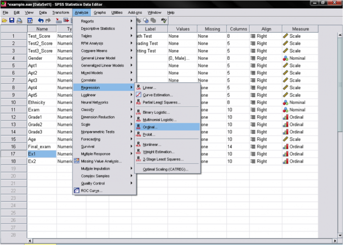
The ordinal regression analysis can be found in Analyze/Regression/Ordinal…
The next dialog box allows us to specify the ordinal regression model. For our example the final exam (four levels – fail, pass, good, distinction) is the dependent variable, the five factors are Ex1 … Ex5 for the five exams taken during the term. Please note that this works correctly only if you define the right measurement scales within SPSS.
SPSS allows including one or more continuous covariates (interval or ratio). However, adding multiple covariates often leads to a large cell probability matrix with many empty cells.
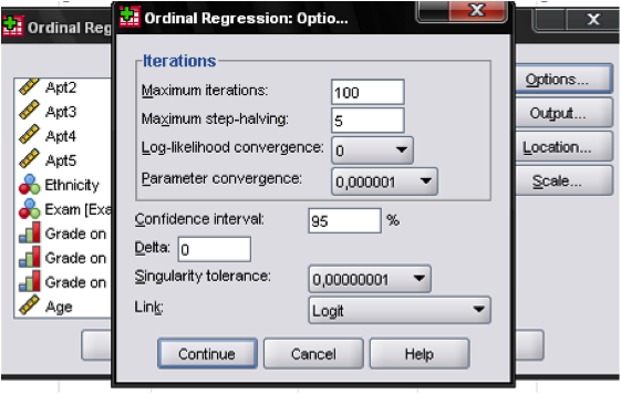
The options dialog lets us manage iteration solution settings and change the link setting for ordinal regression. The link function in ordinal regression transforms the cumulative probabilities of the ordered dependent variable to estimate the model. There are five different link functions.
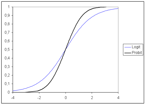
Researchers often use both logit and probit models in ordinal regression, fitting each and choosing the one that fits better. Probit assumes a normal distribution for the dependent variable’s categories, while logit assumes a log distribution. The difference between logit and probit is typically more apparent in small samples.
3. Negative log-log: This link function works best when the probability of the lower category is high. Mathematically, the negative log-log is expressed as p(z) = –log(–log(z)).
4. Complementary log-log: This function is the inverse of the negative log-log function. This function works best when the probability of the higher category is high. Mathematically complementary log-log is p(z) = log (– log (1 – z)).
5. Cauchit: This link function applies when the data contains extreme values. Mathematically Cauchit is p(z) = tan (p(z – 0.5)).
We keep the default settings for ordinal regression and add the test of parallel lines in the Output menu.


