Conduct and Interpret a Multiple Linear Regression
Understanding Multiple Linear Regression
Multiple linear regression predicts and explores relationships between one outcome variable and multiple predictor variables. It’s like solving a puzzle, understanding how different factors influence a specific result.
The Essence of Multiple Linear Regression
Multiple linear regression draws a line through multi-dimensional data to represent the relationship between the dependent and independent variables. It’s like finding the best path through a forest, where the path represents predicted outcomes based on different conditions.
Stages of Multiple Linear Regression Analysis
- Analyzing Data: Before anything, we look at the data to see how the variables relate to each other. Check for patterns or directions in the data, often visualized through scatter plots.
- Estimating the Model: Here, we fit the line—or in more complex cases, a multi-dimensional plane—to the data. This step is about finding the formula that best predicts the outcome based on the predictors.
- Evaluating the Model: Finally, we assess how good our model is. Does it make accurate predictions? Is it useful for the questions we’re trying to answer?
- Casual Analysis: Understanding how changes in predictor variables cause changes in the outcome.
- Forecasting Effects: Predicting how adjustments to predictor variables will affect the outcome.
- Trend Forecasting: Using the model to predict future values and trends based on current data.
Need help conducting your Multiple Linear Regression? Leverage our 30+ years of experience and low-cost same-day service to make progress on your results today!
Schedule now using the calendar below.
Multiple Linear Regression in Practice
Consider a study aiming to predict students’ reading scores on a standardized test based on five different aptitude tests. The first step is to ensure a linear relationship between the aptitude tests (predictor variables) and the reading scores (outcome variable). Generate scatter plots for each predictor against the outcome in SPSS through the Graphs menu.
In SPSS:
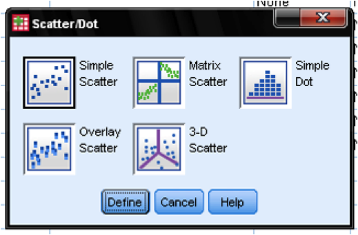
To tackle our research question—can we predict a student’s reading score based on their performance in five aptitude tests?—we start by visually inspecting the relationship between these variables using scatter plots. Generate scatter plots individually for each predictor or use a matrix scatter plot under Graphs > Legacy Dialogs > Scatter/Dot in SPSS. This visual inspection is crucial for confirming that our data meets the assumptions for multiple linear regression, setting the stage for a meaningful analysis.
In essence, multiple linear regression is about understanding and predicting the complex interplay between various factors and an outcome. By methodically analyzing, estimating, and evaluating, it provides a window into the causal relationships and trends that define our world.
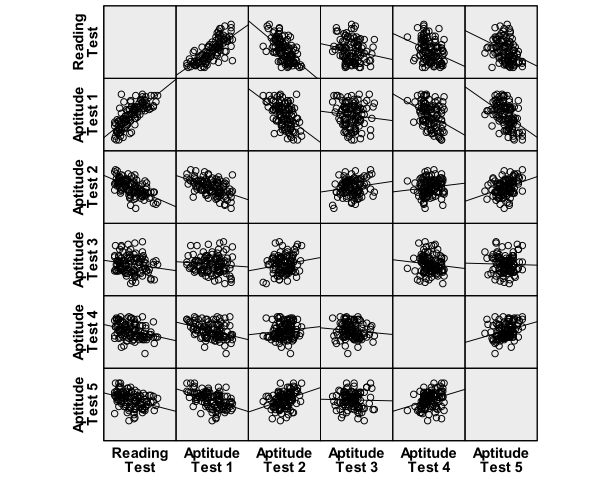
The scatter plots indicate a good linear relationship between writing score and the aptitude tests 1 to 5, where there seems to be a positive relationship for aptitude test 1 and a negative linear relationship for aptitude tests 2 to 5.
Multivariate normality
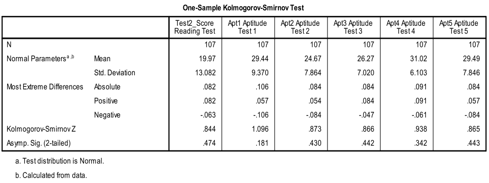
Secondly, we need to check for multivariate normality. This can either be done with an ‘eyeball’ test on the Q-Q-Plots or by using the 1-Sample K-S test to test the null hypothesis that the variable approximates a normal distribution. The K-S test is not significant for all variables, thus we can assume normality.
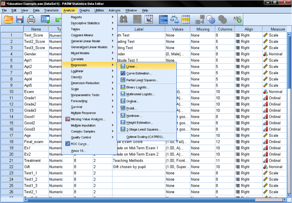
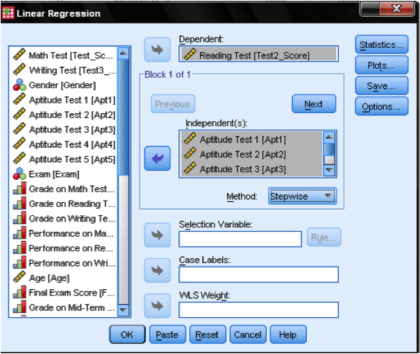
Multiple linear regression is found in SPSS in Analyze/Regression/Linear…
To answer our research question we need to enter the variable reading scores as the dependent variable in our multiple linear regression model and the aptitude test scores (1 to 5) as independent variables. We also select stepwise as the method. The default method for the multiple linear regression analysis is ‘Enter‘, which means that all variables are forced to be in the model. But since over-fitting is a concern of ours, we want only the variables in the model that explain additional variance. Stepwise means that the variables are entered into the regression model in the order of their explanatory power.
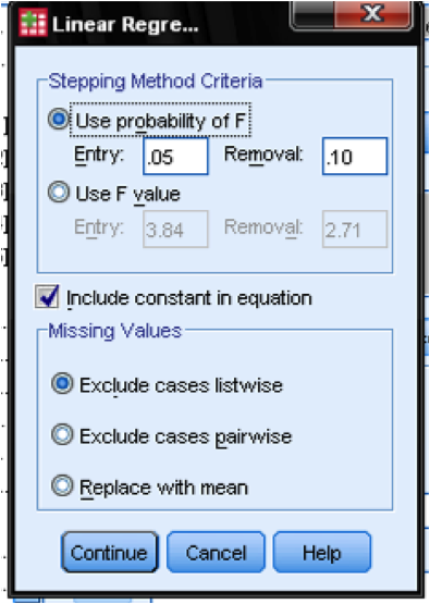
In the field Options… we can define the criteria for stepwise inclusion in the model. Include variables that increase F by at least 0.05 and exclude those that increase F by less than 0.1. This dialog box also allows us to manage missing values (e.g., replace them with the mean).
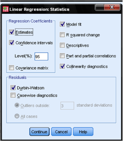
The dialog Statistics… allows us to include additional statistics that we need to assess the validity of our linear regression analysis. Even though it is not a time series, we include Durbin-Watson to check for autocorrelation and we include the collinearity that will check for autocorrelation.
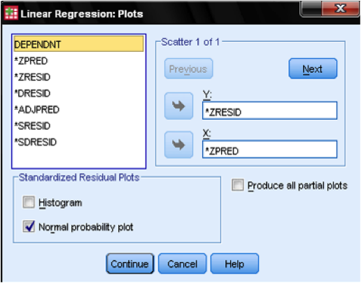
In the dialog Plots…, we add the standardized residual plot (ZPRED on x-axis and ZRESID on y-axis), which allows us to eyeball homoscedasticity and normality of residuals.
