The Linear Regression Analysis in SPSS
This example is based on the FBI’s 2006 crime statistics. Particularly we are interested in the relationship between size of the state and the number of murders in the city.
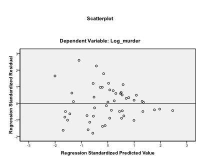
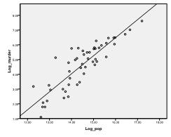
First we need to check whether there is a linear relationship in the data. We first check the scatterplot, which indicates a good linear relationship. Therefore, we can conduct a linear regression analysis. Furthermore, we check Pearson’s Bivariate Correlation and find that both variables are highly correlated (r = .959, p < 0.001).
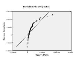
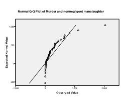
Secondly we need to check for multivariate normality. In our example we find that multivariate normality might not be present.
The Kolmogorov-Smirnov test confirms this suspicion (p = 0.002 and p = 0.006). Conducting a ln-transformation on the two variables fixes the problem and establishes multivariate normality (K-S test p = .991 and p = .543).
Need help conducting your Linear Regression Analysis? Leverage our 30+ years of experience and low-cost same-day service to complete your results today!
Schedule now using the calendar below.
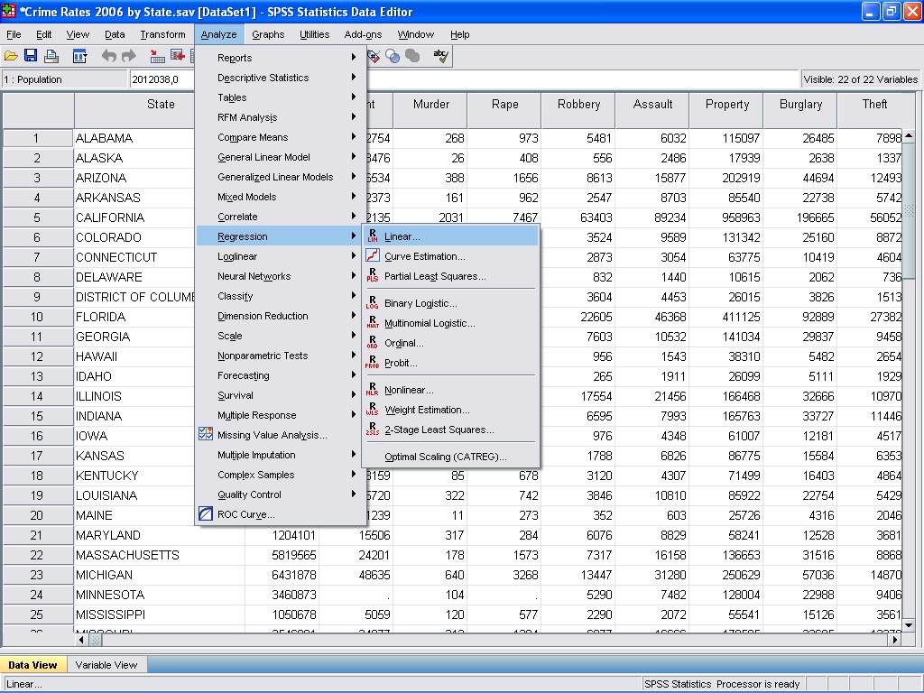
We now can conduct the linear regression analysis. Linear regression is found in SPSS in Analyze/Regression/Linear…
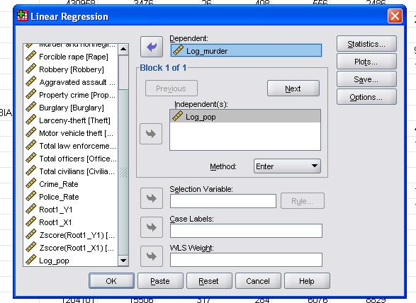
In this simple case we need to just add the variables log_pop and log_murder to the model as dependent and independent variables.
The field statistics allows us to include additional statistics that we need to assess the validity of our linear regression analysis.
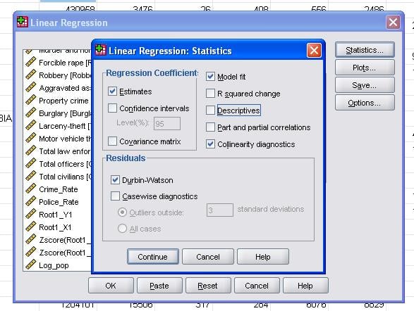
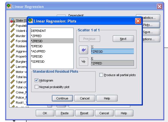
It is advisable to additionally include the collinearity diagnostics and the Durbin-Watson test for auto-correlation. To test the assumption of homoscedasticity of residuals we also include a special plot in the Plots menu.
The SPSS Syntax for the linear regression analysis is
REGRESSION
/MISSING LISTWISE
/STATISTICS COEFF OUTS R ANOVA COLLIN TOL
/CRITERIA=PIN(.05) POUT(.10)
/NOORIGIN
/DEPENDENT Log_murder
/METHOD=ENTER Log_pop
/SCATTERPLOT=(*ZRESID ,*ZPRED)
/RESIDUALS DURBIN HIST(ZRESID).
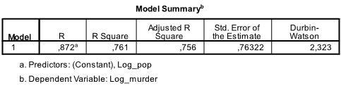
The output’s first table shows the model summary and overall fit statistics. The adjusted R² is 0.756, with R² = 0.761, meaning the linear regression explains 76.1% of the data variance. The Durbin-Watson d = 2.323, between 1.5 and 2.5, indicating no first-order linear auto-correlation in the data.
The next table shows the F-test. The null hypothesis of the F-test is that there is no linear relationship between the variables (R² = 0). With F = 156.2 and 50 df, the test is significant, indicating a linear relationship between the variables.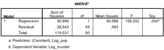
The next table shows the regression coefficients, intercept, and their significance in the model. We find that our linear regression analysis estimates the linear regression function to be y = -13.067 + 1.222
* x. Note that this does not mean 1.2 additional murders per 1,000 inhabitants, as we ln-transformed the variables.
If we re-ran the linear regression analysis with the original variables we would end up with y = 11.85 + 6.7*10-5 which shows that for every 10,000 additional inhabitants we would expect to see 6.7 additional murders.
In our linear regression analysis the test tests the null hypothesis that the coefficient is 0. The t-test finds that both intercept and variable are highly significant (p < 0.001) and thus we might say that they are different from zero.
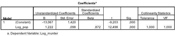
This table also includes the Beta weights (which express the relative importance of independent variables) and the collinearity statistics. However, since we have only 1 independent variable in our analysis we do not pay attention to those values.
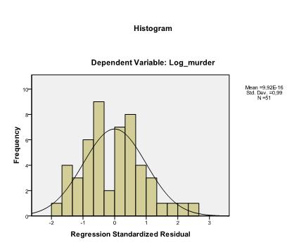
The last thing we need to check is the homoscedasticity and normality of residuals. The histogram indicates that the residuals approximate a normal distribution. The Q-Q-Plot of z*pred and z*presid shows us that in our linear regression analysis there is no tendency in the error terms.