Paired Sample T-Test
The Paired Sample T-Test Looks Simple. That’s Why It Trips Up So Many Dissertations.
Here’s what happens: you run a pre-test/post-test design, you get a significant p-value, you write it up, and your committee sends it back. Why? Because you didn’t check normality on the differences. Or you reported p < .05 instead of the exact p-value. Or you left out the effect size. The paired t-test is the most common analysis in dissertation research; and the one students most often report incompletely. Not because they can’t do it, but because they think it’s too simple to get wrong.
The tipping point in your results chapter isn’t the analysis itself. It’s the assumptions, the effect size, and the way you report it. Miss any one of those, and what felt like a straightforward chapter becomes a revision cycle.
The difference between a t-test that gets approved and one that gets sent back is about 30 minutes of assumption testing and proper APA reporting. That’s the tipping point. Don’t miss it.

Get Expert Help with Your Results. Schedule Your Free Consultation.
20 minutes with Dr. Lani. No obligation. No pressure.
The paired sample t-test, sometimes called the dependent sample t-test, is a statistical procedure. Specifically, it determines whether the mean difference between two sets of observations is zero. In a paired sample t-test, one should measure each subject or entity twice, resulting in pairs of observations. Common applications of the paired sample t-test include case-control studies or repeated-measures designs. Suppose if you want to evaluate the effectiveness of a company training program, you might follow the following approach. One approach you might consider would be to measure the performance of a sample of employees before and after completing the program, and analyze the differences using a paired sample t-test.
Hypotheses
Like many statistical procedures, the paired sample t-test has two competing hypotheses, the null hypothesis and the alternative hypothesis. The null hypothesis assumes that the true mean difference between the paired samples is zero. Under this model, all observable differences are explained by random variation. Conversely, the alternative hypothesis assumes that the true mean difference between the paired samples is not equal to zero. As a result, the alternative hypothesis can take one of several forms depending on the expected outcome. If the direction of the difference does not matter, one should use a two-tailed hypothesis. Otherwise, the power of the test increases by an upper-tailed or lower-tailed hypothesis. The null hypothesis remains the same for each type of alternative hypothesis. The paired sample t-test hypotheses are formally defined below:
• The true mean difference (\(\mu_d\)) poses to be equal to zero in the null hypothesis (\(H_0\)).
• A two-tailed alternative hypothesis (\(H_1\)) believes that the true mean difference \(\mu_d\) is not equal to zero.
• According to an upper-tailed alternative hypothesis (\(H_1\)) the true mean difference \(\mu_d\) is greater than zero.
• It is assumed that \(\mu_d\) is lesser than zero in a lower-tailed alternative hypothesis (\(H_1\)).
Note. It is important to remember that hypotheses are never about data, they are about the processes which produce the data. In the formulas above, the value of \(\mu_d\) is unknown. The goal of hypothesis testing is to determine the hypothesis (null or alternative) with which the data are more consistent.
Need help conducting your paired t-test? Leverage our 30+ years of experience and low-cost, same-day service to complete your results today!
Schedule now using the calendar below.
Assumptions
As a parametric procedure (a procedure which estimates unknown parameters), the paired sample t-test makes several assumptions. Although t-tests are quite robust, it is good practice to evaluate the degree of deviation from these assumptions in order to assess the quality of the results. In a paired sample t-test, the observations are defined as the differences between two sets of values. Hence, each assumption refers to these differences, and not the original data values. The paired sample t-test has four main assumptions:
- • The dependent variable must be continuous (interval/ratio).
- • The observations are independent of one another.
- • The dependent variable should approximately distribute normally.
- • The dependent variable should not contain any outliers.
Level of Measurement
As the paired sample t-test is based on the normal distribution, it requires the sample data to be numeric and continuous. So, the continuous data can take on any value within a range (income, height, weight, etc.). The opposite of continuous data is discrete data, which can only take on a few values (Low, Medium, High, etc.). Occasionally, one can use discrete data to approximate a continuous scale, such as with Likert-type scales.
Independence
You usually cannot test the independence of observations, but you can reasonably assume it if the data collection process was random and without replacement. In our example, it is reasonable to assume that the participating employees are independent of one another.
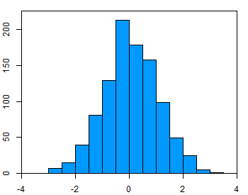
Normality
To test the assumption of normality, a variety of methods are available, but the simplest is to inspect the data visually using a tool like a histogram (Figure 1). Real-world data are almost never perfectly normal, so the consideration of this assumption reasonably met if the shape looks approximately symmetric and bell-shaped. The data in the example figure below approximately follows a normal distribution.
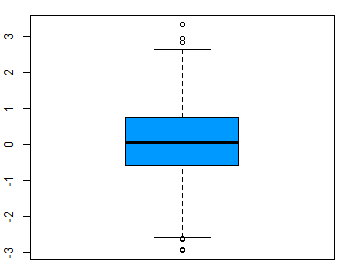
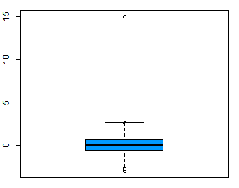
Outliers
Outliers are rare values that appear far away from the majority of the data. They can bias the results and potentially lead to incorrect conclusions if not handled properly. One method for dealing with outliers is to simply remove them. However, removing data points can introduce other types of bias into the results, and potentially result in losing critical information. If outliers seem to have a lot of influence on the results, a nonparametric test such as the Wilcoxon Signed Rank Test may be appropriate to use instead. Boxplot can help to identify outliers (Figure 2).
Procedure
The procedure for a paired sample t-test involves four steps. The following are the symbols that should be used:
- \(D\ =\ \)Differences between two paired samples
- \(d_i\ =\ \)The \(i^{th}\) observation in \(D\)
- \(n\ =\ \)The sample size
- \(\overline{d}\ =\ \)The sample mean of the differences
- \(\hat{\sigma}\ =\ \)The sample standard deviation of the differences
- \(T\ =\)The critical value of a t-distribution with (\(n\ -\ 1\)) degrees of freedom
- \(t\ =\ \)The t-statistic (t-test statistic) for a paired sample t-test
- \(p\ =\ \)The \(p\)-value (probability value) for the t-statistic.
The following are the four steps:
- 1. Calculate the sample mean.
- \(\overline{d}\ =\ \cfrac{d_1\ +\ d_2\ +\ \cdots\ +\ d_n}{n}\)
- 2. Calculate the sample standard deviation.
- \(\hat{\sigma}\ =\ \sqrt{\cfrac{(d_1\ -\ \overline{d})^2\ +\ (d_2\ -\ \overline{d})^2\ +\ \cdots\ +\ (d_n\ -\ \overline{d})^2}{n\ -\ 1}}\)
- 3. Calculate the test statistic.
- \(t\ =\ \cfrac{\overline{d}\ -\ 0}{\hat{\sigma}/\sqrt{n}}\)
- 4. Calculate the probability of observing the test statistic under the null hypothesis. This value is obtained by comparing t to a t-distribution with (\(n\ -\ 1\)) degrees of freedom. This can be done by looking up the value in a table, such as those found in many statistical textbooks, or with statistical software for more accurate results.
- \(p\ =\ 2\ \cdot\ Pr(T\ >\ |t|)\) (two-tailed)
- \(p\ =\ Pr(T\ >\ t)\) (upper-tailed)
- \(p\ =\ Pr(T\ <\ t)\) (lower-tailed)
Determine whether the results provide sufficient evidence to reject the null hypothesis in favor of the alternative hypothesis.
Interpretation
There are two types of significance to consider when interpreting the results of a paired sample t-test, statistical significance and practical significance.
Statistical Significance
The p-value determines the Statistical significance. The p-value gives the probability of observing the test results under the null hypothesis. The lower the p-value, the lower the probability of obtaining a result like the one that was observed if the null hypothesis was true. Thus, a low p-value indicates decreased support for the null hypothesis. However, the possibility that the null hypothesis is true and that we simply obtained a very rare result can never be ruled out completely. The cutoff value for determining statistical significance is ultimately decided on by the researcher, but usually a value of .05 or less is chosen. This corresponds to a 5% (or less) chance of obtaining a result like the one that was observed if the null hypothesis was true.
Practical Significance
Practical significance depends on the subject matter specifically. It is not uncommon, especially with large sample sizes, to observe a result that is statistically significant but not practically significant. In most cases, both types of significance are required in order to draw meaningful conclusions.