How to Conduct Logistic Regression

Logistic Regression Analysis estimates the log odds of an event.  If we analyze a pesticide, it either kills the bug or it does not.  Thus we have a dependent variable that has two values 0 = bug survives, 1 = bug dies.  We vary the composition of the pesticide in 5 factors.  Basically it is the concentration of 5 different poisons (Lethane, Pyrethrum, Piperonyl Butoxide, D.D.T. and Chlordane) in the spray.

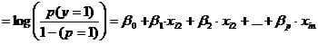
The second step of logistic regression is to formulate the model, i.e. that variable X1, X2, and X3 have a causal influence on the probability of event Y to happen and that their relationship is linear.  We can now express the logistic regression function as logit(p)

The third step of regression analysis is to fit the regression line using maximum likelihood estimation.  Maximum likelihood is an iterative approach to maximize the likelihood function.  SPSS specifically -2*log(likelihood function) ? min!

Linear regression analysis uses least squares to estimate the coefficients.  Generally both methods calculate the same results and both methods are equal if the residuals are normally distributed.

Let’s assume that our model just looks at the concentration of Lethane in the bug spray.  The maximum likelihood estimator established the function that logit(p) = -1.4 + 2.0*x where x is the amount of lethane in the spray.

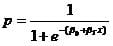
Now the probability of killing the bug p is

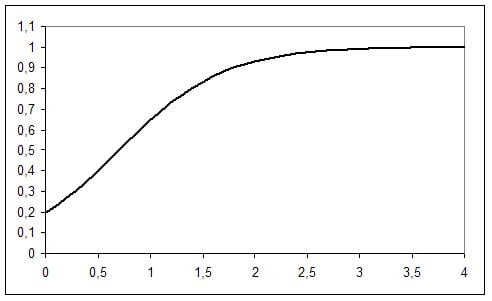
This gives us the following graph

The critical cut-off value is p=0.5 in our example that corresponds with the critical value 0.7 for the concentration in the spray.

We also know that 2.0 is our coefficient for the Lethane concentration.  That means that 2.0 * p * (1-p) is the slope of the curve.  So when p = 0.5 an additional unit of Lethane changes the probability by 0.5.  Note that this is not linearly constant for all values if p = 0.8 the probability changes by 0.32 (2.0 * 0.8 * 0.2).  This is because the log odds ratio stays constant.  The log odds is not an intuitive concept, but since it is the log of the odds ratio = log (p/(1-p)) we simply can translate this result back into odds ratios with exp(x).  That is in our case exp(2.0), which is 7.39. Therefore increasing the Lethane concentration by one unit the odds of killing the bug are multiplied by 7.39.  This is the same as saying that for two configurations of our spray the one with the higher concentration of Lethane has a +639% higher probability of killing the bug than the one with the lower concentration of Lethane.

When it come to predicting the dichotomous dependent variable (bug is either dead or alive) then the cut-off is drawn at p = 0.5. This is at p > 0.5 we expect the bug to be dead.  The critical concentration for this to happen is

which is in this example 1.4/2.0 = 0.7.
The last step is to check the validity of the logistic regression model.  Similar to regular regression analysis we calculate a R².  However for logistic regression this is called a Pseudo-R².  The measures of fit are based on the -2log likelihood, which is the minimization criteria for the maximum likelihood estimation.

The first R² value of the logistic regression is Cox & Snell’s R² (although other Pseudo R² exists, we focus on the 2 that are part of SPSS).

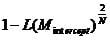
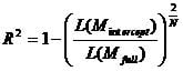
This R² expresses the improvement of the full model with all variables included over the Block 0 model, that only includes the intercept. Theoretically L(M) is the conditional probability of y = 1 for a given x.  With N observations of the probability of y=1 in our data, L(M) = pn.  Thus if we draw the nth root gives us the approximate of the likelihood of each y value.  However the maximum value of Cox & Snell’s R² is not 1, it is

which is < 1.

Thus Nagelkerke’s R² corrects this by dividing the Cox & Snell R² by

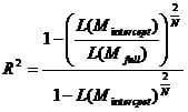
that is

However if the full model does not improve compared to the intercept model R² > 0.

Related Pages:

• What is Logistic Regression