Testing Normality in SPSS
You have set the methodological stage, entered your data, and you are getting ready to run those fancy analyses you have been anticipating (or dreading) all this time. If you have already read our overview on some of SPSS’s data cleaning and management procedures, you should be ready to get started. But wait! You are using a parametric analysis, and you know that stats book you read said something about normality. It is important, but what is it, and how do you know if your data follows normality? Well, first it is important to know what kind of normality you are looking for. There are two main types: univariate and multivariate.
Here we will talk about univariate normality. This goes along with the concept of the bell curve, which is the depiction of data with a lot of “middle-ground” scores, but only a few high or low scores. This follows the figure here, where the vertical (y) axis represents the number of people (or observations) with low, average, and high scores.

Discover How We Assist to Edit Your Dissertation Chapters
Aligning theoretical framework, gathering articles, synthesizing gaps, articulating a clear methodology and data plan, and writing about the theoretical and practical implications of your research are part of our comprehensive dissertation editing services.
- Bring dissertation editing expertise to chapters 1-5 in timely manner.
- Track all changes, then work with you to bring about scholarly writing.
- Ongoing support to address committee feedback, reducing revisions.
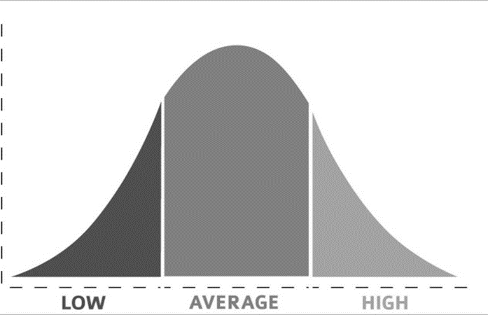
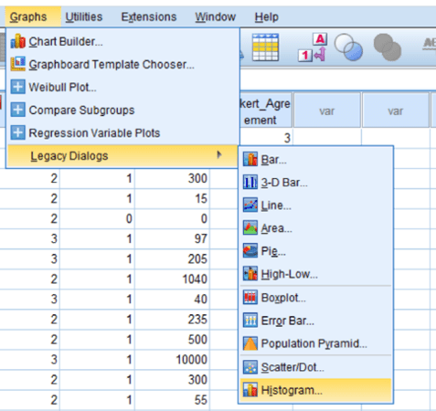
A few deviations from this distribution can exist. For example, the hump can be pushed to one side or the other, resulting in skew. A high skew can mean there are disproportionate numbers of high or low scores. On the other hand, platykurtosis and leptokurtosis happen when the hump is either too flat or too tall (respectively). You can start by looking at a figure like the one above in SPSS by selecting Graphs > Legacy dialogs > Histogram, and selecting your variable. Clicking OK should show you a chart that looks similar to the one above. If your distribution does not follow a typical bell shape, you might need to dig into the numbers.
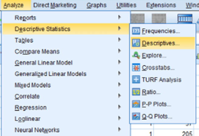
To give some numbers to your distribution, you can also look at the skew and kurtosis values by selecting Analyze > Descriptive Statistics > Descriptives… and dragging over the variables that you want to examine. Clicking on Options… gives you the ability to select Kurtosis and Skewness in the options menu. Hit OK and check for any Skew values over 2 or under -2, and any Kurtosis values over 7 or under -7 in the output. Those values might indicate that a variable may be non-normal.
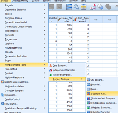
With all that said, there is another simple way to check normality: the Kolmogorov Smirnov, or KS test. This test checks the variable’s distribution against a perfect model of normality and tells you if the two distributions are different. You can reach this test by selecting Analyze > Nonparametric Tests > Legacy Dialogs > and clicking 1-sample KS test. Just make sure that the box for “Normal” is checked under distribution.
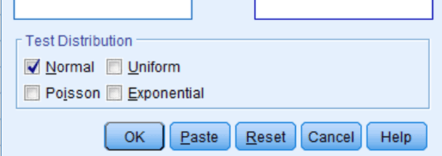

The difference between your distribution and a perfectly normal one is checked based on a p value, and is interpreted just like any other p-value. If the p-value is less than .05, your distribution is significantly different from a normal distribution and might be cause for concern. If it is .05 or higher, there is no significant difference from normality, and your normality-dependent analysis is ready to roll!