Assumptions of Multiple Linear Regression Analysis
Multiple linear regression analysis is predicated on several fundamental assumptions that ensure the validity and reliability of its results. Understanding and verifying these assumptions is crucial for accurate model interpretation and prediction.
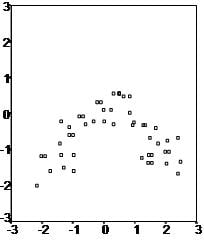
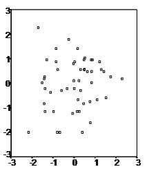
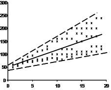
- Linear Relationship: The core premise of multiple linear regression is the existence of a linear relationship between the dependent (outcome) variable and the independent variables. This linearity can be visually inspected using scatterplots, which should reveal a straight-line relationship rather than a curvilinear one.
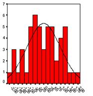
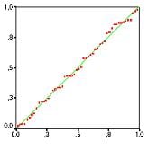
- Multivariate Normality: The analysis assumes that the residuals (the differences between observed and predicted values) are normally distributed. This assumption can be assessed by examining histograms or Q-Q plots of the residuals, or through statistical tests such as the Kolmogorov-Smirnov test.
- No Multicollinearity: It is essential that the independent variables are not too highly correlated with each other, a condition known as multicollinearity. This can be checked using:
- Correlation matrices, where correlation coefficients should ideally be below 0.80.
- Variance Inflation Factor (VIF), with VIF values above 10 indicating problematic multicollinearity. Solutions may include centering the data (subtracting the mean score from each observation) or removing the variables causing multicollinearity.
- Homoscedasticity: The variance of error terms (residuals) should be consistent across all levels of the independent variables. A scatterplot of residuals versus predicted values should not display any discernible pattern, such as a cone-shaped distribution, which would indicate heteroscedasticity. Addressing heteroscedasticity might involve data transformation or adding a quadratic term to the model.
Sample Size and Variable Types: The model requires at least two independent variables, which can be of nominal, ordinal, or interval/ratio scale. A general guideline for sample size is a minimum of 20 cases per independent variable.
First, linear regression needs the relationship between the independent and dependent variables to be linear. It is also important to check for outliers since linear regression is sensitive to outlier effects. The linearity assumption can best be tested with scatter plots, the following two examples depict two cases, where no and little linearity is present.
Need help with your research?
Schedule a time to speak with an expert using the calendar below?
User-friendly Software
Transform raw data to written interpreted APA results in seconds.
Secondly, the linear regression analysis requires all variables to be multivariate normal. This assumption can best be checked with a histogram or a Q-Q-Plot. Normality can be checked with a goodness of fit test, e.g., the Kolmogorov-Smirnov test. When the data is not normally distributed a non-linear transformation (e.g., log-transformation) might fix this issue.
Thirdly, linear regression assumes that there is little or no multicollinearity in the data. Multicollinearity occurs when the independent variables are too highly correlated with each other.
Multicollinearity may be tested with three central criteria:
1) Correlation matrix – when computing the matrix of Pearson’s Bivariate Correlation among all independent variables the correlation coefficients need to be smaller than 1.
2) Tolerance – the tolerance measures the influence of one independent variable on all other independent variables; the tolerance is calculated with an initial linear regression analysis. Tolerance is defined as T = 1 – R² for these first step regression analysis. With T < 0.1 there might be multicollinearity in the data and with T < 0.01 there certainly is.
3) Variance Inflation Factor (VIF) – the variance inflation factor of the linear regression is defined as VIF = 1/T. With VIF > 5 there is an indication that multicollinearity may be present; with VIF > 10 there is certainly multicollinearity among the variables.
If multicollinearity is found in the data, centering the data (that is deducting the mean of the variable from each score) might help to solve the problem. However, the simplest way to address the problem is to remove independent variables with high VIF values.
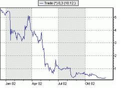
Fourth, linear regression analysis requires that there is little or no autocorrelation in the data. Autocorrelation occurs when the residuals are not independent from each other. For instance, this typically occurs in stock prices, where the price is not independent from the previous price.
4) Condition Index – the condition index is calculated using a factor analysis on the independent variables. Values of 10-30 indicate a mediocre multicollinearity in the linear regression variables, values > 30 indicate strong multicollinearity.
If multicollinearity is found in the data centering the data, that is deducting the mean score might help to solve the problem. Other alternatives to tackle the problems is conducting a factor analysis and rotating the factors to insure independence of the factors in the linear regression analysis.
Fourthly, linear regression analysis requires that there is little or no autocorrelation in the data. Autocorrelation occurs when the residuals are not independent from each other. In other words when the value of y(x+1) is not independent from the value of y(x).
While a scatterplot allows you to check for autocorrelations, you can test the linear regression model for autocorrelation with the Durbin-Watson test. Durbin-Watson’s d tests the null hypothesis that the residuals are not linearly auto-correlated. While d can assume values between 0 and 4, values around 2 indicate no autocorrelation. As a rule of thumb values of 1.5 < d < 2.5 show that there is no auto-correlation in the data. However, the Durbin-Watson test only analyses linear autocorrelation and only between direct neighbors, which are first order effects.
The last assumption of the linear regression analysis is homoscedasticity. The scatter plot is good way to check whether the data are homoscedastic (meaning the residuals are equal across the regression line). The following scatter plots show examples of data that are not homoscedastic (i.e., heteroscedastic):
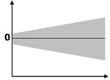
The Goldfeld-Quandt Test can also be used to test for heteroscedasticity. The test splits the data into two groups and tests to see if the variances of the residuals are similar across the groups. If homoscedasticity is present, a non-linear correction might fix the problem.
Related Pages:
Linear Regression-Video Tutorial
Conduct and Interpret a Linear Regression
Statistics Solutions can assist with your quantitative analysis by assisting you to develop your methodology and results chapters. The services that we offer include:
Edit your research questions and null/alternative hypotheses
Write your data analysis plan; specify specific statistics to address the research questions, the assumptions of the statistics, and justify why they are the appropriate statistics; provide references
Justify your sample size/power analysis, provide references
Explain your data analysis plan to you so you are comfortable and confident
Two hours of additional support with your statistician
Quantitative Results Section (Descriptive Statistics, Bivariate and Multivariate Analyses, Structural Equation Modeling, Path analysis, HLM, Cluster Analysis)
Clean and code dataset
Conduct descriptive statistics (i.e., mean, standard deviation, frequency and percent, as appropriate)
Conduct analyses to examine each of your research questions
Write-up results
Provide APA 7th edition tables and figures
Explain chapter 4 findings
Ongoing support for entire results chapter statistics
Please call 727-442-4290 to request a quote based on the specifics of your research, schedule using the calendar on this page, or email [email protected]